3 Exercise and Sleep Analysis
3.1 Introduction
In this chapter, we examined how different forms of exercise affect sleep habits. Participants were divided into four exercise groups (None, Cardio, Weights, and Cardio + Weights), and their average hours of sleep were measured before and after the experiment. Sleep efficiency was also measured at the end of the study. The goal of this analysis was to determine whether certain types of exercise are associated with greater improvements in sleep outcomes. To address this question, we conducted descriptive statistics and visualizations, followed by inferential analyses including t-tests and ANOVAs. These methods allowed us to compare sleep outcomes across exercise groups and identify which exercise method, if any, showed the strongest impact on sleep.
3.3 Setup and Data Import
## [1] "participant_info_midterm" "sleep_data_midterm"participant_info_midterm <- read_xlsx("midterm_sleep_exercise.xlsx", sheet="participant_info_midterm")
sleep_data_midterm <- read_xlsx("midterm_sleep_exercise.xlsx", sheet="sleep_data_midterm")
glimpse(participant_info_midterm)## Rows: 100
## Columns: 4
## $ ID <chr> "P001", "P002", "P003", "P004", "P005", "P006", "P007", "P008", …
## $ Exercise_Group <chr> "NONE", "Nonee", "None", "None", "None", "None", "None", "None",…
## $ Sex <chr> "Male", "Malee", "Female", "Female", "Male", "Female", "Male", "…
## $ Age <dbl> 35, 57, 26, 29, 33, 33, 32, 30, 37, 28, 30, 20, 42, 31, 33, 26, …## Rows: 100
## Columns: 4
## $ ID <chr> "P001", "P002", "P003", "P004", "P005", "P006", "P007", "P008"…
## $ Pre_Sleep <chr> "zzz-5.8", "Sleep-6.6", NA, "SLEEP-7.2", "score-7.4", "Sleep-6…
## $ Post_Sleep <dbl> 4.7, 7.4, 6.2, 7.3, 7.4, 7.1, 6.7, 9.0, 5.1, 6.3, 6.2, 4.6, 7.…
## $ Sleep_Efficiency <dbl> 81.6, 75.7, 82.9, 83.6, 83.5, 88.5, 83.6, 73.4, 88.2, 80.4, 85…We imported the Excel file midterm_sleep_exercise.xlsx, which contained two sheets: participant information (participant_info_midterm) and sleep data (sleep_data_midterm). We used the read_xlsx() function from the readxl package to load each sheet and glimpse() to preview their structures.
The dataset contained 100 participants. The participant_info_midterm dataset includes the following variables: ID, Exercise_Group, Sex, Age. While the sleep_data_midterm dataset contains: ID, Pre_Sleep, Post_Sleep, Sleep_Efficiency.
3.4 Merge and Base Cleaning
## [1] "ID" "Exercise_Group" "Sex" "Age"## [1] "NONE" "Nonee" "None" "N" "Cardio"
## [6] "C" "WEIGHTZ" "WEIGHTS" "WEIGHTSSS" "Cardio+Weights"
## [11] "CW" "C+W"participant_info_midterm <- participant_info_midterm %>%
mutate(Exercise_Group = case_when(
Exercise_Group %in% c("NONE", "Nonee","N") ~ "None",
Exercise_Group == "C" ~ "Cardio",
Exercise_Group %in% c("WEIGHTZ", "WEIGHTS", "WEIGHTSSS") ~ "Weights",
Exercise_Group %in% c("CW", "C+W") ~ "Cardio+Weights",
TRUE ~ Exercise_Group))
unique(participant_info_midterm$Sex)## [1] "Male" "Malee" "Female" "Femalee" "F" "M" "Fem" "MALE"
## [9] "Mal"participant_info_midterm <- participant_info_midterm %>%
mutate(Sex = case_when(
Sex %in% c("Malee", "MALE", "Mal", "M") ~ "Male",
Sex %in% c("Femalee", "Fem", "F") ~ "Female",
TRUE ~ Sex))
midterm_data_combined<- merge(participant_info_midterm, sleep_data_midterm, by="ID")Once the data were imported, we standardized the Exercise_Group and Sex variable labels to ensure consistency across the dataset. This was done by recoding inconsistent entries in the Exercise_Group and Sex columns to unified category names (e.g., “cardio” and “CARDIO” → “Cardio”; “m” and “MALE” → “Male”). These adjustments help prevent grouping and categorization errors during analysis.
After cleaning these variables, we merged the two datasets by theID column to create a single dataset, midterm_data_combined, which contains each participant’s demographic information and sleep data. The cleaned and merged dataset now contains the following variables: ID, Exercise_Group, Sex, Age, Pre_Sleep, Post_Sleep, Sleep_Efficiency.
3.5 Create Derived Variables
## [1] "ID"               "Exercise_Group"   "Sex"              "Age"
## [5] "Pre_Sleep" "Post_Sleep" "Sleep_Efficiency"## Rows: 100
## Columns: 7
## $ ID <chr> "P001", "P002", "P003", "P004", "P005", "P006", "P007", "P008"…
## $ Exercise_Group <chr> "None", "None", "None", "None", "None", "None", "None", "None"…
## $ Sex <chr> "Male", "Male", "Female", "Female", "Male", "Female", "Male", …
## $ Age <dbl> 35, 57, 26, 29, 33, 33, 32, 30, 37, 28, 30, 20, 42, 31, 33, 26…
## $ Pre_Sleep <chr> "zzz-5.8", "Sleep-6.6", NA, "SLEEP-7.2", "score-7.4", "Sleep-6…
## $ Post_Sleep <dbl> 4.7, 7.4, 6.2, 7.3, 7.4, 7.1, 6.7, 9.0, 5.1, 6.3, 6.2, 4.6, 7.…
## $ Sleep_Efficiency <dbl> 81.6, 75.7, 82.9, 83.6, 83.5, 88.5, 83.6, 73.4, 88.2, 80.4, 85…midterm_data_combined <- midterm_data_combined %>%
mutate(Pre_Sleep = str_extract(Pre_Sleep, "\\d+\\.?\\d*"),
Pre_Sleep = as.numeric(Pre_Sleep))
midterm_data_combined <- midterm_data_combined %>%
mutate(Sleep_Difference = Post_Sleep - Pre_Sleep)
midterm_data_combined <- midterm_data_combined %>%
mutate(AgeGroup2 = case_when(
Age < 40 ~ "<40",
Age >= 40 ~ ">=40"))
sum(is.na(midterm_data_combined$Sleep_Difference))## [1] 14After cleaning and merging the data, we created several derived variables to prepare the dataset for analysis. First, we cleaned the Pre_Sleep variable by extracting the numeric values and converting them to a numeric format. We then created a new variable, Sleep_Difference, which represents the change in average hours of sleep from before to after the experiment.
We also created a new variable to separate participants into two age groups: those under 40 (<40) and those aged 40 or older (≥40). Lastly, we removed any missing values from Sleep_Difference to ensure accurate statistical analyses. The dataset now contains 86 rows.
3.6 Descriptive Statistics
3.6.1 Summary of Sleep Difference and Sleep Efficiency
sleep_summary <- rbind(cbind(Variable = "Sleep_Difference",
  favstats(~ Sleep_Difference, data = midterm_data_combined)),
  cbind(Variable = "Sleep_Efficiency",
  favstats(~ Sleep_Efficiency, data = midterm_data_combined)))

kable(sleep_summary,
caption = "Descriptive statistics for sleep difference and sleep efficiency across all participants. This table summarizes central tendency and variability for changes in sleep duration and overall sleep efficiency following the exercise intervention.")| Variable | min | Q1 | median | Q3 | max | mean | sd | n | missing |
|---|---|---|---|---|---|---|---|---|---|
| Sleep_Difference | -1.1 | 0.300 | 0.75 | 1.100 | 2.1 | 0.6825581 | 0.6610494 | 86 | 0 |
| Sleep_Efficiency | 71.7 | 79.975 | 83.30 | 88.425 | 101.5 | 83.7755814 | 5.9738043 | 86 | 0 |
Overall, participants showed an average Sleep_Difference of 0.68 hours (SD = 0.66), indicating a small increase in sleep from before to after the experiment. The Sleep_Efficiency variable had a mean of 83.78% (SD = 5.97), suggesting relatively high sleep efficiency across participants.
3.6.2 Group-Wise Summary of Sleep Difference and Efficiency
execrise_sleep_summary <- rbind(
  cbind(Varible = "Sleep_Difference",
        favstats(Sleep_Difference ~ Exercise_Group, data = midterm_data_combined)),
  cbind(Varible = "Sleep_Efficiency",
        favstats(Sleep_Efficiency ~ Exercise_Group, data = midterm_data_combined))) %>%
  arrange(desc(mean))

kable(execrise_sleep_summary,
caption = "Group-wise descriptive statistics for sleep difference and sleep efficiency by exercise group. This table compares average changes in sleep duration and overall sleep efficiency across the four exercise conditions.")| Varible | Exercise_Group | min | Q1 | median | Q3 | max | mean | sd | n | missing |
|---|---|---|---|---|---|---|---|---|---|---|
| Sleep_Efficiency | Cardio+Weights | 74.5 | 83.50 | 88.7 | 90.5 | 96.3 | 86.8347826 | 5.9803169 | 23 | 0 |
| Sleep_Efficiency | Cardio | 75.9 | 81.30 | 85.5 | 88.0 | 101.5 | 85.4476190 | 5.9916291 | 21 | 0 |
| Sleep_Efficiency | Weights | 74.8 | 77.90 | 80.8 | 83.6 | 89.5 | 81.4571429 | 4.3113306 | 21 | 0 |
| Sleep_Efficiency | None | 71.7 | 76.60 | 81.5 | 83.6 | 90.4 | 81.0714286 | 5.5514992 | 21 | 0 |
| Sleep_Difference | Cardio | 0.3 | 0.70 | 1.2 | 1.4 | 2.1 | 1.1380952 | 0.4852589 | 21 | 0 |
| Sleep_Difference | Cardio+Weights | -0.1 | 0.65 | 0.9 | 1.1 | 1.5 | 0.8608696 | 0.3822649 | 23 | 0 |
| Sleep_Difference | Weights | -0.7 | 0.30 | 0.5 | 1.1 | 1.8 | 0.6666667 | 0.6126445 | 21 | 0 |
| Sleep_Difference | None | -1.1 | -0.40 | 0.1 | 0.6 | 0.9 | 0.0476190 | 0.6384505 | 21 | 0 |
When comparing group-wise means by Exercise_Group for both Sleep_Difference and Sleep_Efficiency, participants in the Cardio+Weights (M = 86.83%) and Cardio (M = 85.45%) groups showed the highest average sleep efficiency. In contrast, the None group had the lowest sleep efficiency average (M = 81.07%).
Similarly, for Sleep_Difference, the Cardio group showed the largest average increase in sleep (M = 1.14), followed by the Cardio+Weights group (M = 0.86), while the None group showed minimal change (M = 0.05). Based on these descriptive results, cardio-based exercise groups tend to show higher average sleep efficiency and greater increases in sleep duration.
3.7 Visulization (3 plots)
3.7.1 Boxplot: Sleep_Difference ~ Exercise_Group
midterm_data_combined$Exercise_Group <- factor(midterm_data_combined$Exercise_Group,
                                            levels = c("None", "Cardio", "Weights", "Cardio+Weights"))

ggplot(midterm_data_combined, aes(x = Exercise_Group, y = Sleep_Difference))+
  geom_boxplot(fill = "lightblue", color = "black")+
  labs(title = "Sleep difference by exercise group",
       x = "Type of Exercise",
       y ="Sleep Difference (hours)") +
theme_minimal(base_size = 12) +
  theme(
    plot.title   = element_text(size = 17, family = "serif", face = "bold"),
    axis.title.x = element_text(size = 12, family = "serif"),
    axis.title.y = element_text(size = 12, family = "serif")
  )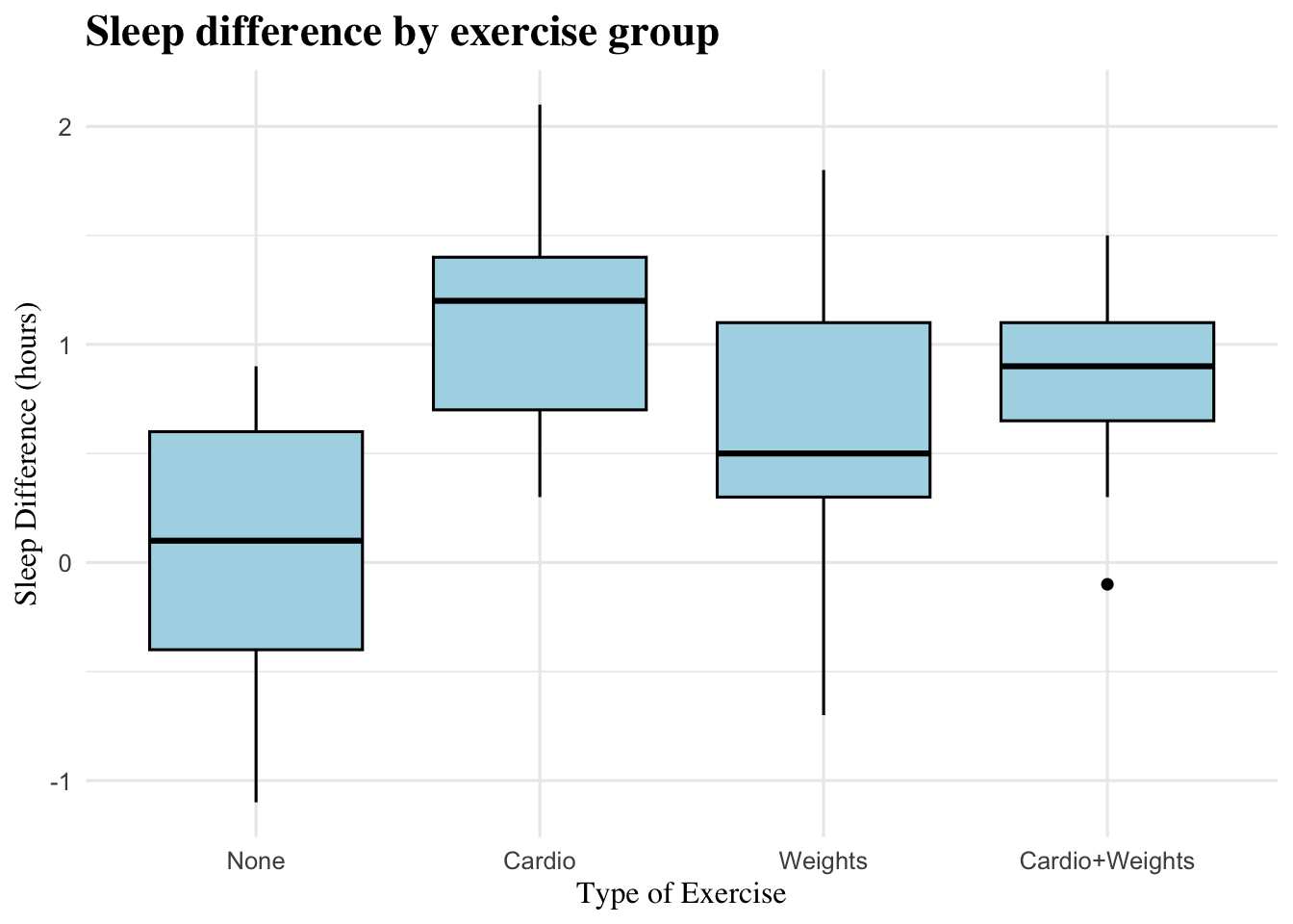
(#fig:boxplot diff-group)Boxplot showing the distribution of sleep difference (post–pre sleep hours) across exercise groups (None, Cardio, Weights, Cardio+Weights). This figure illustrates how changes in sleep duration vary by type of exercise.
3.7.1.1 Interpretation:
The boxplot above shows how Sleep_Difference varied across the four exercise groups. Overall, participants in the Cardio group exhibited the greatest improvements in sleep duration, Followed by Cardio+Weights group. The Weights group showed little improvement, while the None group had the lowest and most spread-out results, meaning their sleep changes were smaller and less consistent. Overall, the plot suggests that cardio-based exercise groups were associated with larger increases in sleep duration compared to the other exercise conditions..
3.7.2 Boxplot: Sleep_Efficiency ~ Exercise_Group
ggplot(midterm_data_combined, aes(x = Exercise_Group, y = Sleep_Efficiency))+
  geom_boxplot(fill = "cadetblue", color = "black")+
  labs(title = "Sleep efficiency by exercise group",
       x = "Type of Exercise",
       y ="Sleep Efficiency") +
theme_minimal(base_size = 12) +
  theme(
    plot.title   = element_text(size = 17, family = "serif", face = "bold"),
    axis.title.x = element_text(size = 12, family = "serif"),
    axis.title.y = element_text(size = 12, family = "serif")
  )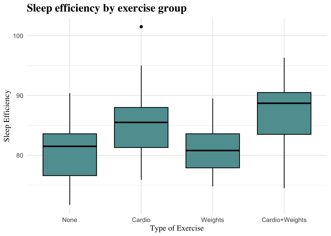
Figure 3.1: Boxplot showing sleep efficiency across the four exercise groups. This figure illustrates differences in sleep efficiency by type of exercise.
3.7.2.1 Interpretation:
The boxplot above shows how Sleep_Efficiency varied across the four exercise groups. Overall, participants in the Cardio+Weights group showed the highest sleep efficiency, followed by the Cardio group. The Weights group had lower efficiency, while the None group showed the lowest and most variable results. Overall, the plot suggests that cardio-based or combined exercise is associated with higher sleep efficiency.
3.7.3 Scatterplot: Sleep_Difference ~ Sleep_Efficiency (with trend line)
ggplot(midterm_data_combined, aes(x = Sleep_Efficiency, y = Sleep_Difference))+
  geom_point(color="steelblue")+
  geom_smooth(method = "lm", color = "darkblue")+
  labs(title = "Relationship between sleep efficiency and sleep difference ",
       x = "Sleep Efficiency",
       y ="Sleep Difference (hours)") +
theme_minimal(base_size = 12) +
  theme(
    plot.title   = element_text(size = 17, family = "serif", face = "bold"),
    axis.title.x = element_text(size = 12, family = "serif"),
    axis.title.y = element_text(size = 12, family = "serif")
  )
## `geom_smooth()` using formula = 'y ~ x'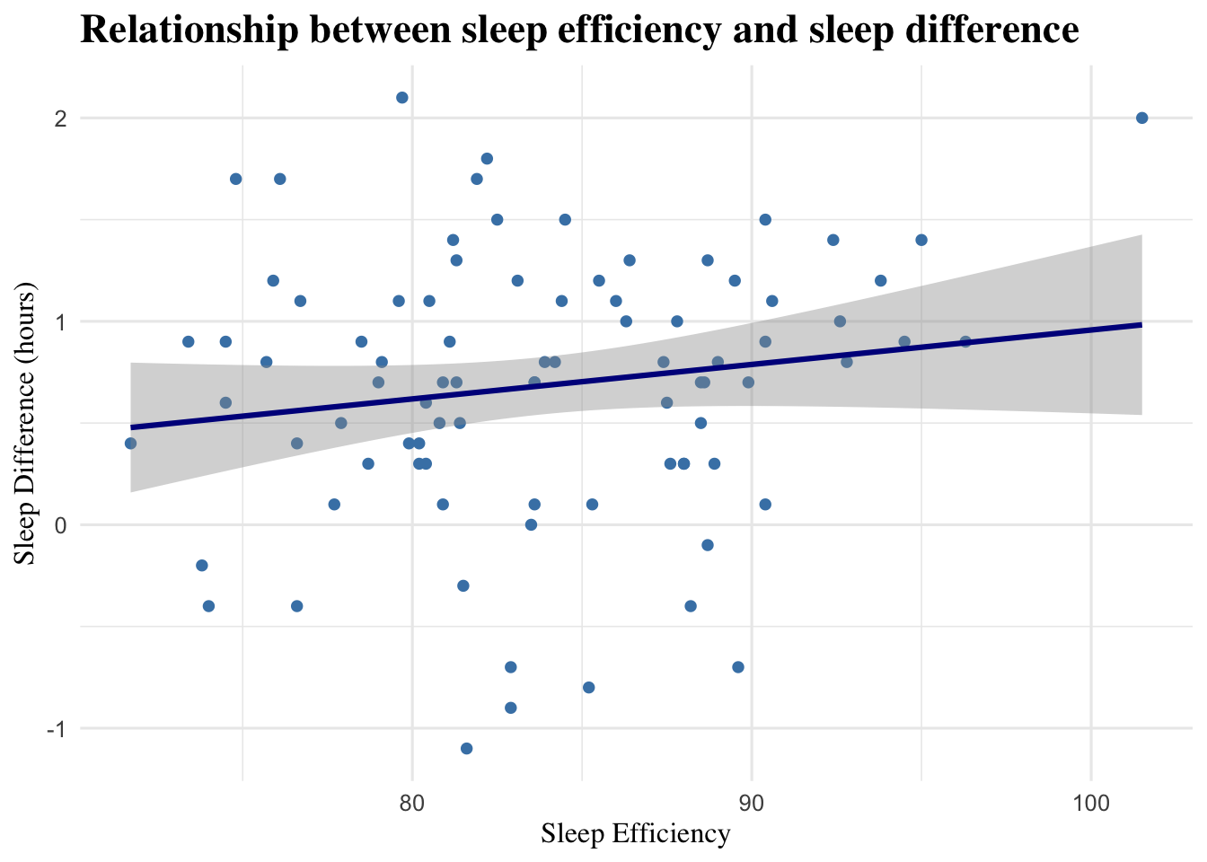
Figure 3.2: Scatterplot showing the relationship between sleep efficiency and sleep difference, with a fitted linear trend line. This figure illustrates how changes in sleep efficiency relate to changes in sleep duration.
3.7.3.1 Interpretation:
The scatterplot above shows the relationship between Sleep_Efficiency and Sleep_Difference. The slight upward trend suggests that participants with higher sleep efficiency also tended to show greater improvements in sleep duration. However, the points are relatively spread out, indicating that the relationship is weak. Overall, this suggests that while better sleep efficiency may be linked to longer sleep, the connection is not very strong or consistent across participants.
3.8 T-Tests
3.8.1 Sleep_Difference ~ Sex
##
##  Welch Two Sample t-test
##
## data:  Sleep_Difference by Sex
## t = 1.5801, df = 77.647, p-value = 0.1182
## alternative hypothesis: true difference in means between group Female and group Male is not equal to 0
## 95 percent confidence interval:
##  -0.05865017  0.50972574
## sample estimates:
## mean in group Female   mean in group Male
##            0.7795918            0.5540541
3.8.1.1 Interpretation:
Based on the t-test comparing sleep differences between the two sex groups (Male vs. Female), females (M = 0.78) had a slightly higher average sleep difference than males (M = 0.55). However, this difference was not statistically significant, t(77.65) = 1.58, p = 0.118. Since the p-value is greater than the significance level of 0.05, it means that there’s a greater chance that the difference we observed is by random chance. Hence, there’s not enough evidence to conclude that sleep change differs by sex.
3.8.2 Sleep_Difference ~ AgeGroup2
##
##  Welch Two Sample t-test
##
## data:  Sleep_Difference by AgeGroup2
## t = -1.3746, df = 36.662, p-value = 0.1776
## alternative hypothesis: true difference in means between group <40 and group >=40 is not equal to 0
## 95 percent confidence interval:
##  -0.50676303  0.09717936
## sample estimates:
##  mean in group <40 mean in group >=40
##          0.6373134          0.8421053
3.8.2.1 Interpretation:
Based on the t-test comparing sleep difference between the two age groups (<40 or >=40), those who are 40 and older (M=0.84) had slightly higher average sleep difference than those who are younger than 40 (M=0.64). However, this difference was not statistically significant, t(36.66)= -1.37, p=0.178. Once again, the p value appears to be larger than 0.05 threshold for significance, therefore the difference between sleep difference and age groups is not significant.
3.9 ANOVA & Post-Hoc Tests
3.9.1 Sleep_Difference ~ Exercise_Group
anova_difference <- aov(Sleep_Difference ~ Exercise_Group, data = midterm_data_combined)
summary(anova_difference)
## Df Sum Sq Mean Sq F value Pr(>F)
## Exercise_Group 3 13.56 4.520 15.72 3.67e-08 ***
## Residuals 82 23.58 0.288
## ---
## Signif. codes: 0 '***' 0.001 '**' 0.01 '*' 0.05 '.' 0.1 ' ' 1## Analysis of Variance Table (Type III SS)
## Model: Sleep_Difference ~ Exercise_Group
##
## SS df MS F PRE p
## ----- --------------- | ------ -- ----- ------ ----- -----
## Model (error reduced) | 13.560 3 4.520 15.717 .3651 .0000
## Error (from model) | 23.583 82 0.288
## ----- --------------- | ------ -- ----- ------ ----- -----
## Total (empty model) | 37.144 85 0.437## Tukey multiple comparisons of means
## 95% family-wise confidence level
##
## Fit: aov(formula = Sleep_Difference ~ Exercise_Group, data = midterm_data_combined)
##
## $Exercise_Group
## diff lwr upr p adj
## Cardio-None 1.0904762 0.6564482 1.52450413 0.0000000
## Weights-None 0.6190476 0.1850197 1.05307556 0.0018927
## Cardio+Weights-None 0.8132505 0.3887628 1.23773822 0.0000171
## Weights-Cardio -0.4714286 -0.9054565 -0.03740063 0.0278779
## Cardio+Weights-Cardio -0.2772257 -0.7017134 0.14726203 0.3237562
## Cardio+Weights-Weights 0.1942029 -0.2302848 0.61869060 0.62872943.9.1.1 Interpretation:
The one-way ANOVA revealed a significant effect of Exercise_Group on Sleep_Difference, F(3, 82) = 15.72, p < .001. The PRE value of 0.37 suggests that Exercise_Group explained about 37% of the total variance in Sleep_Difference.
Post-hoc Tukey tests showed that the Cardio (p < .001), Weights (p = .0019), and Cardio+Weights (p < .001) groups each had significantly greater improvements in sleep compared to the None group. The Cardio group also showed a significantly greater increase in sleep compared to the Weights group (p = .028). However, differences between Cardio+Weights vs. Cardio (p = .324) and Cardio+Weights vs. Weights (p = .629) were not statistically significant.
3.9.2 Sleep_Efficiency ~ Exercise_Group
anova_efficiency <- aov(Sleep_Efficiency ~ Exercise_Group, data = midterm_data_combined)
summary(anova_efficiency)
## Df Sum Sq Mean Sq F value Pr(>F)
## Exercise_Group 3 540.4 180.1 5.925 0.00104 **
## Residuals 82 2492.9 30.4
## ---
## Signif. codes: 0 '***' 0.001 '**' 0.01 '*' 0.05 '.' 0.1 ' ' 1## Analysis of Variance Table (Type III SS)
## Model: Sleep_Efficiency ~ Exercise_Group
##
## SS df MS F PRE p
## ----- --------------- | -------- -- ------- ----- ----- -----
## Model (error reduced) | 540.400 3 180.133 5.925 .1782 .0010
## Error (from model) | 2492.939 82 30.402
## ----- --------------- | -------- -- ------- ----- ----- -----
## Total (empty model) | 3033.339 85 35.686## Tukey multiple comparisons of means
## 95% family-wise confidence level
##
## Fit: aov(formula = Sleep_Efficiency ~ Exercise_Group, data = midterm_data_combined)
##
## $Exercise_Group
## diff lwr upr p adj
## Cardio-None 4.3761905 -0.08623232 8.8386133 0.0566544
## Weights-None 0.3857143 -4.07670851 4.8481371 0.9958617
## Cardio+Weights-None 5.7633540 1.39901844 10.1276896 0.0046379
## Weights-Cardio -3.9904762 -8.45289899 0.4719466 0.0962888
## Cardio+Weights-Cardio 1.3871636 -2.97717203 5.7514992 0.8383629
## Cardio+Weights-Weights 5.3776398 1.01330416 9.7419753 0.00942673.9.2.1 Interpretation:
The one-way ANOVA revealed a significant effect of Exercise_Group on Sleep_Efficiency, F(3, 82) = 5.93, p = .001. The PRE value of 0.18 means that Exercise_Group explained about 18% of the total variance in Sleep_Efficiency.
Post-hoc Tukey tests showed that the Cardio+Weights group had significantly higher sleep efficiency compared to the None group (p = .0046). The difference between the Cardio and None groups was marginally significant (p = .057), suggesting a possible trend toward better sleep efficiency among those in the Cardio group. Other pairwise comparisons, including Weights vs. None (p = .996), Weights vs. Cardio (p = .096), and Cardio+Weights vs. Cardio (p = .839), were not statistically significant.
3.10 Synthesis & Recommendation
After considering both ANOVA and post-hoc tests outcomes, I would recommend Cardio as the exercise regimen to improve overall sleep. The one-way ANOVA showed a significant effect of exercise group on sleep difference, F(3, 82) = 15.72, p < .001, with the exercise group explaining a substantial proportion of variance (37%) in sleep difference. Tukey post-hoc tests revealed that the Cardio group had significantly greater improvements in sleep compared to both the None (p < .05) and Weights (p = .028) groups. Although the Cardio+Weights group also improved sleep, its results were not significantly higher than Cardio alone (p > .05). Similarly, Cardio showed the highest gains in sleep efficiency, making it the best option for improving overall sleep.
3.11 Reflection
I think the most challenging part about this midterm was making sure I transferred everything correctly when moving my code from the R script to R Markdown, especially because I prefer completing the script first. This time around, I felt more confident about writing the actual script and I’m becoming more familiar with the functions. Next time, I want to spend more time reviewing the results of my statistical tests to make sure I fully understand the meaning of each test so I can communicate the findings more effectively.